ArXiv Dives

Greg Schoeninger

Mar 12, 2024

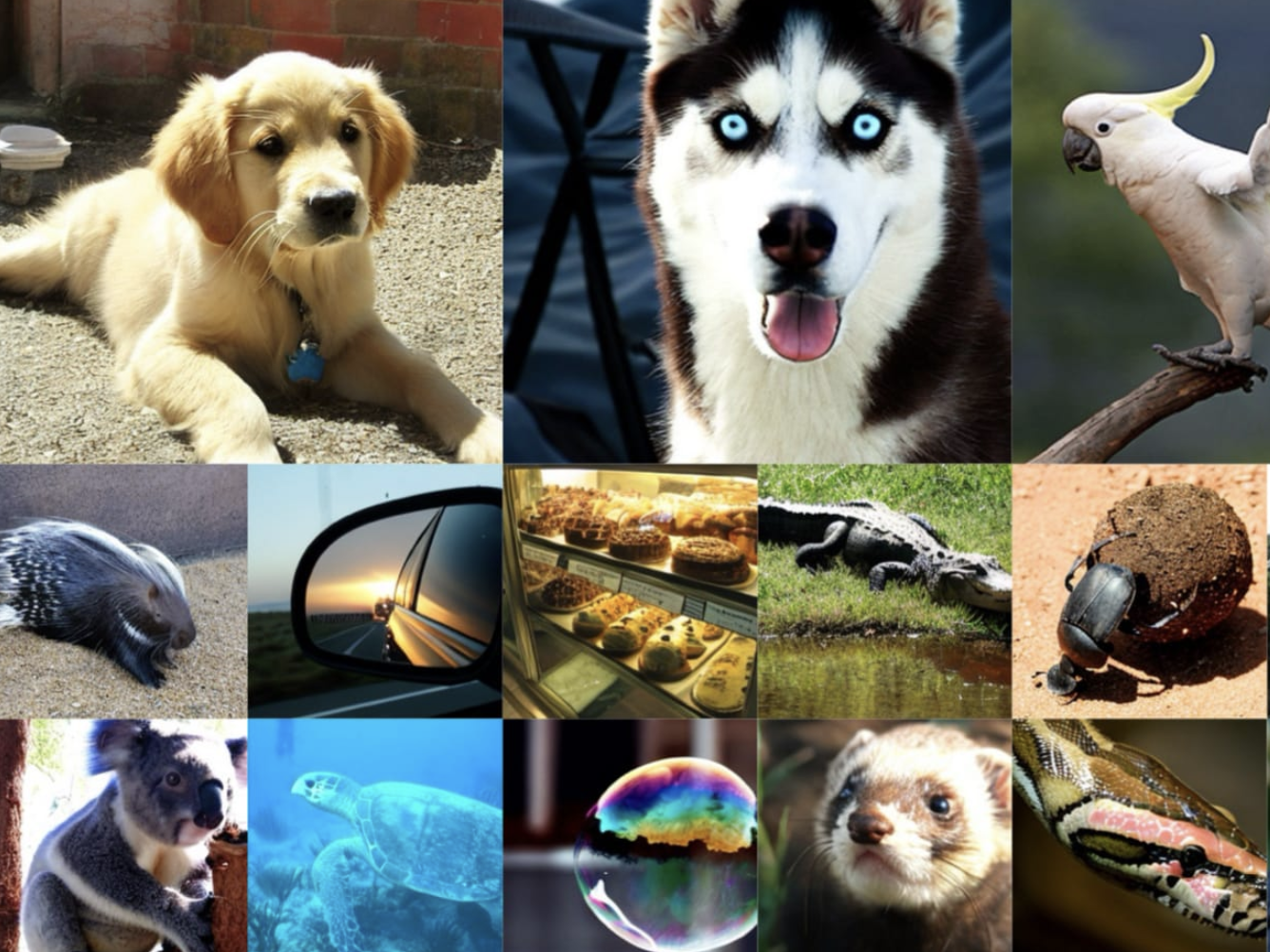
Diffusion transformers achieve state-of-the-art quality generating images by replacing the commonly used U-Net backbone with a transformer that operates on latent patches. They recently gained a lot of hype with the release of the Sora Technical Report that stated that the core model architecture for Sora is a Diffusion Transformer.

Teams: UC Berkeley, NYU

Publish Date: March 2nd, 2023

Scalable Diffusion Models with Transformers

We explore a new class of diffusion models based on the transformer architecture. We train latent diffusion models of images, replacing the commonly-used U-Net backbone with a transformer that operates on latent patches. We analyze the scalability of our Diffusion Transformers (DiTs) through the lens of forward pass complexity as measured by Gflops. We find that DiTs with higher Gflops -- through increased transformer depth/width or increased number of input tokens -- consistently have lower FID. In addition to possessing good scalability properties, our largest DiT-XL/2 models outperform all prior diffusion models on the class-conditional ImageNet 512x512 and 256x256 benchmarks, achieving a state-of-the-art FID of 2.27 on the latter.

arXiv.orgWilliam Peebles

Every Friday at Oxen.ai we host a paper club called "ArXiv Dives" to make us smarter Oxen 🐂 🧠. We believe diving into the details of research papers is the best way to build fundamental knowledge, spot patterns and keep up with the bleeding edge.

These are the notes from our live session, feel free to follow along with the video for context. If you would like to join live to ask questions or join the discussion we would love to have you! Sign up below 👇

Introduction

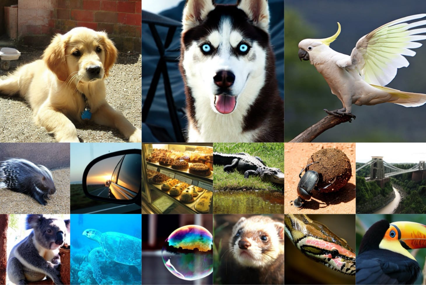
While transformers have taken the machine learning world by storm for many tasks in natural language processing, computer vision and several other domains, for some reason image generation models had remained holdouts on the trend. Prior state of the art image generation models these days are what’s called “diffusion models”.

Popular diffusion models such as “Stable Diffusion” use a convolutional U-Net architecture as their backbone.

This work on Diffusion Transformers shows that the inductive biases that come from Convolution, ResNets, and U-Nets are not crucial to the performance of diffusion models. You can replace the components inside a diffusion model with a transformer and have nice properties such as scalability, robustness, and efficiency.

What is a U-Net?

A U-Net is a type of neural network architecture that can be visualized as a U. It down samples an image to a latent space, then upsamples an output back to the same size as the original image. The latent spaces are connected by skip connections that allow information to flow nicely through the model. In the case of diffusion networks the output is a predicted set of noise, but U-Nets are commonly used in tasks like semantic segmentation image augmentation where the input has to be the same size of the output.

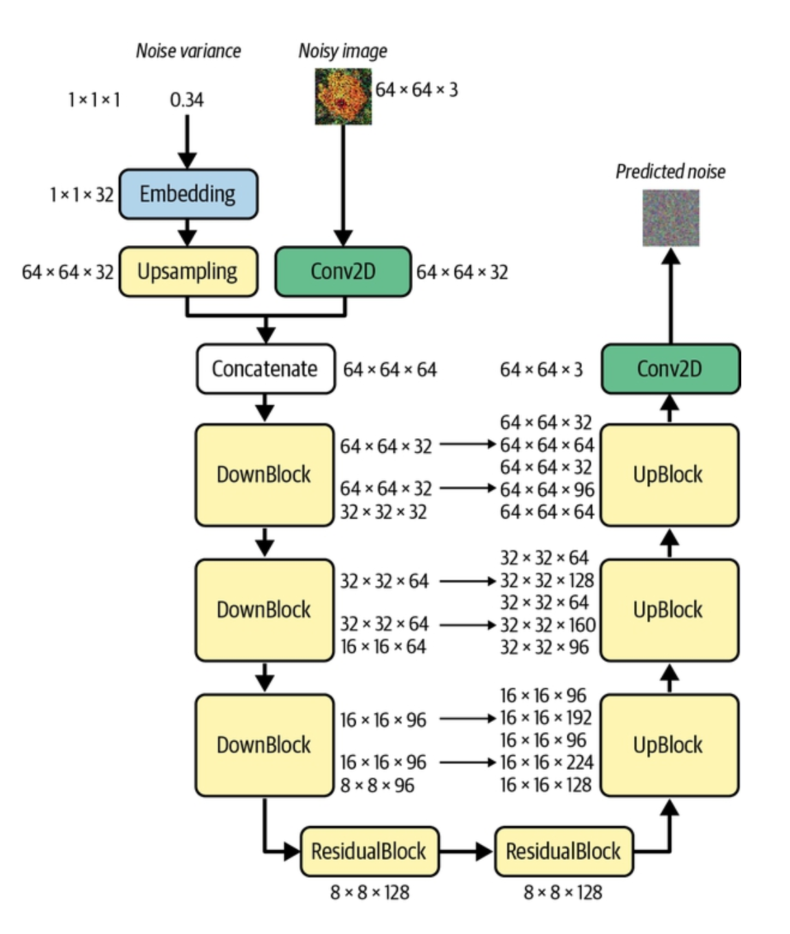
I recommend this source for a lot of the background needed for this post: https://www.amazon.com/Generative-Deep-Learning-Teaching-Machines/dp/1492041947. It covers U-Nets, VAEs, and Diffusion models in detail with great visuals and code.

What is a Diffusion Model?

A "Diffusion Model" in is any type of model that reconstructs images from noise. What is interesting about them is the data augmentation used in training. They use a trick of of slowly applying Gaussian noise to the training images at different time steps, until you end up with something that looks like the image on the right of just fuzzy noise.

Then a neural network is trained to predict the noise at each time step. Each time it predicts the noise, you subtract it from the image, and slowly a realistic image emerges. Kind of like black magic that this works at all.

This paper shows that you can swap out a U-Net with a Vision Transformer (ViT) to end up with a model they call the Diffusion Transformer (DiT).

Throughout the paper they have two metrics that they are optimizing for:

1) Network complexity (the compute used in terms of GFlops)

2) Sample Quality (how good the images look, measured in FID)

Network Complexity

It is common to use parameter count to estimate neural network architecture complexity. This paper argues that parameter count can be a poor proxy for complexity because it does not account for image resolution.

The larger the image, the more compute you typically need.

Whether you are using VIT patches or convolutions, the larger the image, the more surface area it has to cover. Because of this, they look at complexity in terms of Gflops (Giga Floating Point Operations) instead of pure parameter count.

Fréchet inception distance (FID)

The charts later in the paper that assess image quality are measured in a number called FID. This is a numeric metric that computes how well the distribution of generated images match the distribution of real images. Rather than comparing pixels directly to pixels with mean squared error, FID compares the mean and standard deviation of the deepest layer in a pre-trained Inception V-3 model. Keep this in mind as reading the results in the experiments seciton.

Variational Auto Encoder (VAE)

The first step in the Diffusion Transformer model is a VAE. Training a full diffusion model directly in pixel space can be computationally expensive.

Auto encoders can take any data - in this case images - and learn to compress it into a smaller representation (often a single vector of numbers, but could be set of numbers) and then learn to decompress it into the original data or image.

For example, you could take the “FashionMnist” dataset which is 28x28 black and white images of clothes (like the pants above) and compress it all the way down to 4 floating point numbers

[6.3,-0.9]

And have the network learn to reconstruct the image from those 2 numbers.

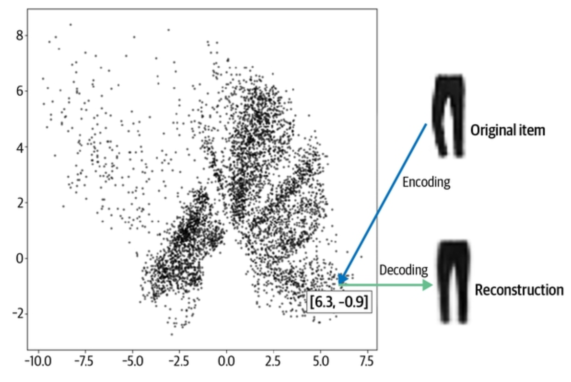
What’s cool about these is you can train them on pretty much unlimited data because you do not need a human in the loop labeling each image.

There is an encoder half of an auto encoder E and a decoder have D.

In their case they use a VAE or Variational Auto Encoder, but the mental model is roughly the same. VAEs help with the problem of "mode collapse" by spreading out the latents into a more well distributed space.

Latent Diffusion Models

Once you have an auto-encoder trained, now you can train a diffusion model on the latent space vectors instead of the pixels of the raw images. Training the diffusion model to predict noise in the latent space is much more efficient than doing it in pixel space, because the latent space is much smaller.

E & D of the auto-encoder are typically frozen in this process, but you can apply the same method of adding noise to the latent space, predicting the noise in the latent space, and using the decoder D to decode the de-noised latent vector.

For the Diffusion Transformer model they use an “off the shelf” Convolutional Variational Auto Encoder, which is the same one used in the Stable Diffusion Models.

This means that a DiT is actually a hybrid of ConvNets and Transformers when you look under the hood, not purely transformers 😄

Diffusion Transformer Architecture

Putting it all together!

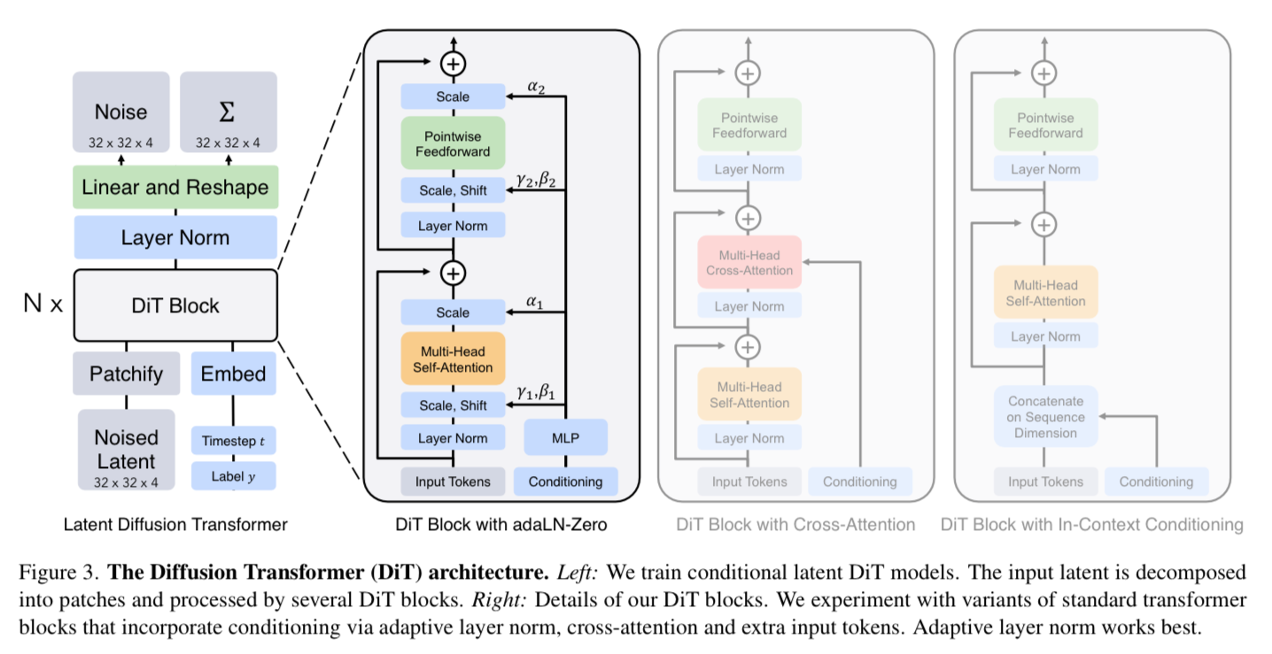
The starting difference between a U-Net and a Transformer is the way the network processes the images. A U-Net does convolutions across the image, where as Transformers chop the image into patches that can be processed and attended to in parallel.

If you are not familiar with Transformers or Vision Transformers I would recommend checking out our past deep dive on them.

The input to the DiT is a 256x256x3 image which is run through a variational auto-encoder which turns it into 32x32x4 latent space z. The latent space is then “patchified” and flattened into a sequence as input into the ViT. They try patch sizes of 2,4, and 8.

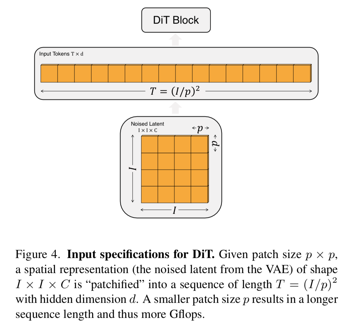
Above would be a patch size of 8, which turns into 4x4 patches (since there is a width and height of 32x32) or a sequence of 16.

They use standard sine-cosine positional embeddings to encode the location of the patch into the input since it is now in a sequence and not spatially arranged.

Changing the patch size has a big affect on the total compute in terms of GFlops, but does not impact the total parameter count. They say that halving p will at least quadruple the GFlops.

DiT Block Design

At a high level, the self-attention in a transformer allows each patch to look at each other patch in the image and relay information to one another. Along with the image patches themselves, they add in additional conditional information at this stage such as noise time steps t, class labels c, and eventually natural language.

They do a few variations of the architecture to see what works best (reference figure 3 above).

In Context Conditioning

To add in the additional information, they simply append t and c as additional tokens in the input sequence and treat them the same as image tokens.

t = denoising timestep

c = class index of the image (cat, dog, bird, etc)

Cross-attention block

Instead of adding t and c as additional tokens in the input sequence, they treat them as a separate sequence of length 2, then add additional cross-attention to the separate sequence. This causes 15% overhead in GFlops because of the additional attention.

Adaptive layer norm (adaLN)

Layer normalization is the process of making sure all the values within a layer are within a certain range (usually 0-1 or with zero mean and unit variance). This helps the network learn faster and be more stable training. Adaptive layer norm learns parameters gamma and beta to perform the normalization.

AdaLN-Zero block

They also learn a scaling parameter alpha applied immediately prior to any residual connections that helps guide how much information from the original input is passed through to the next layer.

Transformer Decoder

After the final DiT block, they need to decode the sequence of image tokens into a prediction of noise / a diagonal covariance prediction. They use a standard linear and reshape layers to do the decoding.

Model Sizes

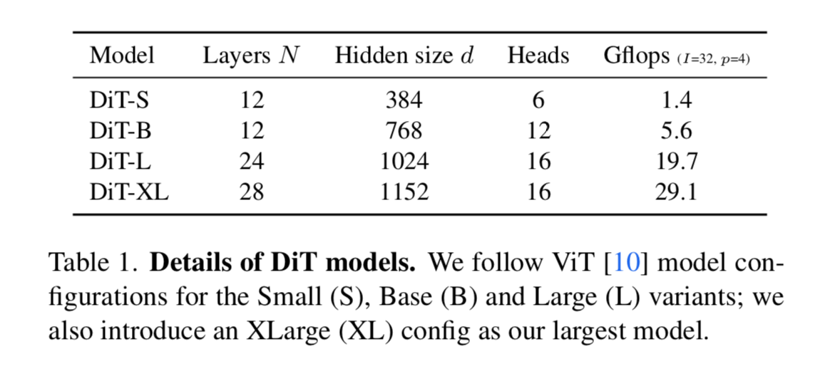
Experimental Results

They evaluate using the FID metric and report FID-50k using 250 DDPM sampling steps. The best model consistently was the adaLN-Zero DiT blocks.

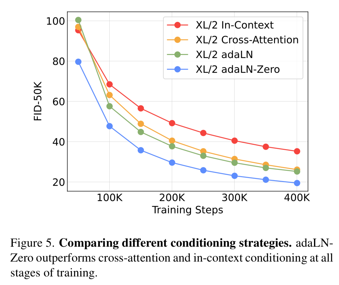
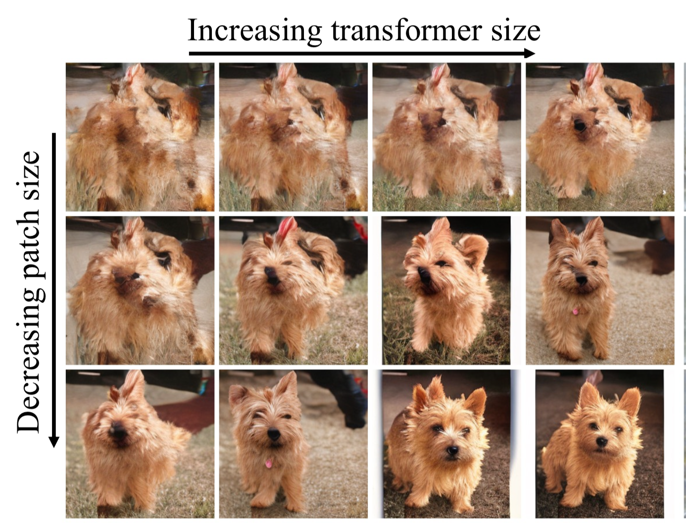
The biggest takeaway of the result section is that scaling model size and decreasing patch size both yield better results.

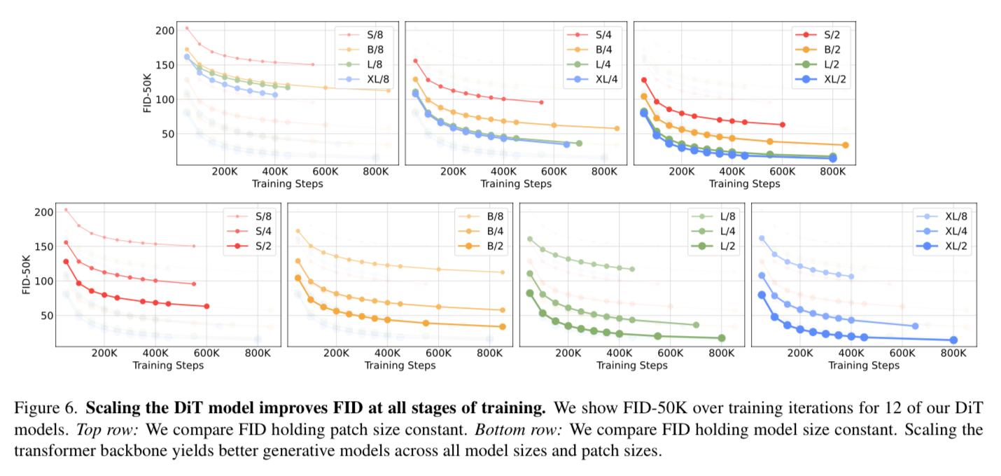
What is interesting is parameter counts do not uniquely determine quality of the DiT model - it is more about the GFlops used.

For example: When model size is held constant and patch size is decreased, the parameter counts are effectively unchanged (in fact, total parameters slightly decrease) but the GFlops increase because you have more patches to process. The models with smaller patch size out perform the models with larger patch size and they claim this is correlated to GFlops.

Small models - even when trained longer, eventually become compute-inefficient relative to larger models trained for fewer steps.

So the smaller the patch size and the larger model the better.

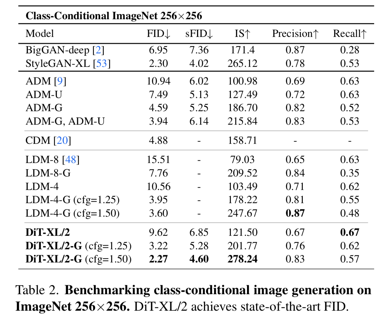
They end up training the DiT-XL/2 for 7M steps to compare it to other models.

Note: The FID score metric was original in GAN research in 2017.

GANs Trained by a Two Time-Scale Update Rule Converge to a Local Nash Equilibrium

Generative Adversarial Networks (GANs) excel at creating realistic images with complex models for which maximum likelihood is infeasible. However, the convergence of GAN training has still not been proved. We propose a two time-scale update rule (TTUR) for training GANs with stochastic gradient descent on arbitrary GAN loss functions. TTUR has an individual learning rate for both the discriminator and the generator. Using the theory of stochastic approximation, we prove that the TTUR converges under mild assumptions to a stationary local Nash equilibrium. The convergence carries over to the popular Adam optimization, for which we prove that it follows the dynamics of a heavy ball with friction and thus prefers flat minima in the objective landscape. For the evaluation of the performance of GANs at image generation, we introduce the “Fréchet Inception Distance” (FID) which captures the similarity of generated images to real ones better than the Inception Score. In experiments, TTUR improves learning for DCGANs and Improved Wasserstein GANs (WGAN-GP) outperforming conventional GAN training on CelebA, CIFAR-10, SVHN, LSUN Bedrooms, and the One Billion Word Benchmark.

arXiv.orgMartin Heusel

The way it works is you take a pre-trained Inception V-3 model and run a real image through, and a generated image through, then look at the activations from the last pooling layer and compare them. If you want full details on the implementation check out these resources.

https://machinelearningmastery.com/how-to-implement-the-frechet-inception-distance-fid-from-scratch/

https://github.com/openai/guided-diffusion/tree/main/evaluations

The problems with this are we are using an image classification model trained on ImageNet meaning its features are only really going to know about objects that are well represented in that dataset. So it is not surprising that a generative model also trained on image net performs well. FID would probably not be a good metric to test out of domain performance for a model.

Qualitative Results

In general, the qualitative results from the model are super impressive.

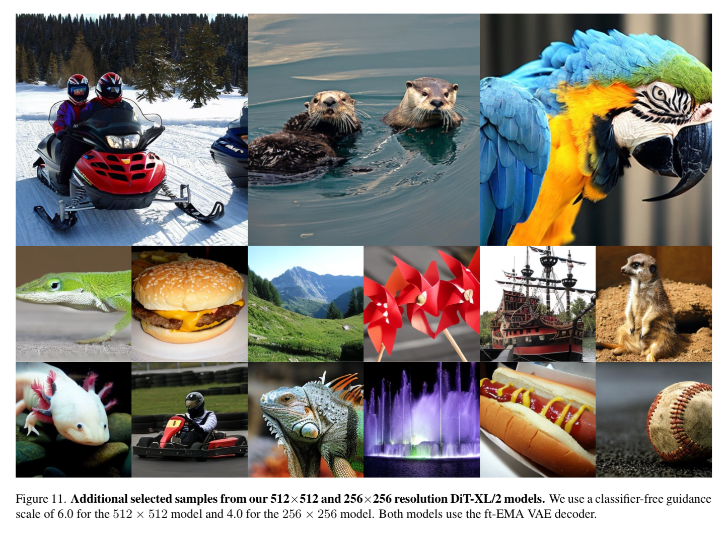
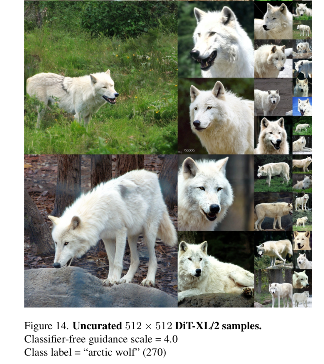
But there are some fun errors if you look closely. Such as...arctic wolf eating rock?

Or demonic faces in the background of images?

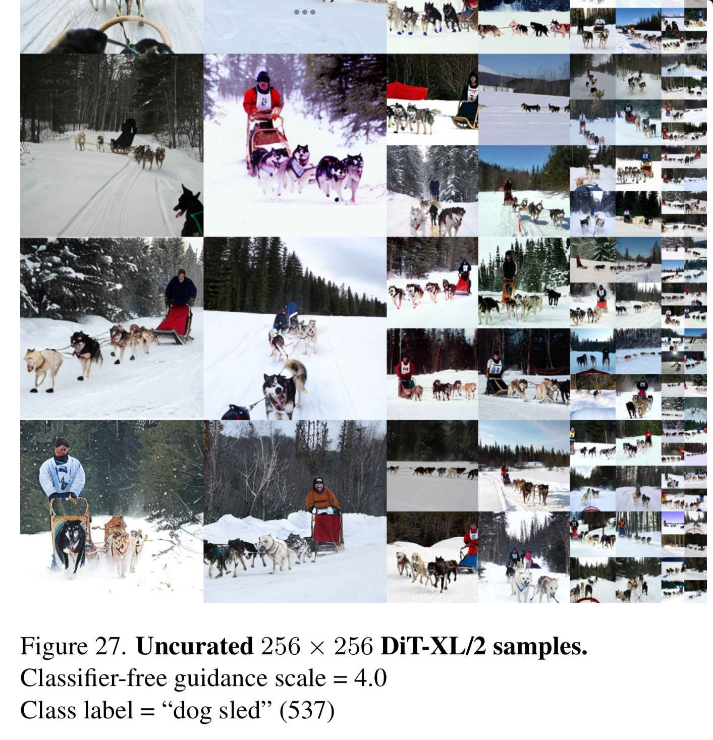
There are many more example in the appendix of the paper if you are interested.

Conclusion

The diffusion transformer paper shows that the inductive biases of traditional U-Nets are not crucial to the performance. If you scale up compute by increasing model size and decreasing patch size, Diffusion Transformers become state of the art image generation models.

In the Sora technical report they mention that the model is a “Diffusion Transformer”. They do not go into the exact technical details but you can imagine they added the time dimension to the patches and had the diffusion process not only sample latent spatial latent spaces in width and height, but also in the time dimension.

The closest paper I saw in the references to what they described in the technical report is a model called WALT from Google.

Photorealistic Video Generation with Diffusion Models

We present W.A.L.T, a transformer-based approach for photorealistic video generation via diffusion modeling. Our approach has two key design decisions. First, we use a causal encoder to jointly compress images and videos within a unified latent space, enabling training and generation across modalities. Second, for memory and training efficiency, we use a window attention architecture tailored for joint spatial and spatiotemporal generative modeling. Taken together these design decisions enable us to achieve state-of-the-art performance on established video (UCF-101 and Kinetics-600) and image (ImageNet) generation benchmarks without using classifier free guidance. Finally, we also train a cascade of three models for the task of text-to-video generation consisting of a base latent video diffusion model, and two video super-resolution diffusion models to generate videos of $512 \times 896$ resolution at $8$ frames per second.

arXiv.orgAgrim Gupta

We will cover WALT in a future dive.

If anyone is up for the challenge - It would be fun to try to implement one of these models and make some of the results reproducible on a smaller scale. The authors of the paper speculate that the Sora model may not be that large (even though it is probably trained on a massive dataset).

Here's my take on the Sora technical report, with a good dose of speculation that could be totally off. First of all, really appreciate the team for sharing helpful insights and design decisions – Sora is incredible and is set to transform the video generation community.

What we… pic.twitter.com/XbxFmgPKxT
— Saining Xie (@sainingxie) February 16, 2024

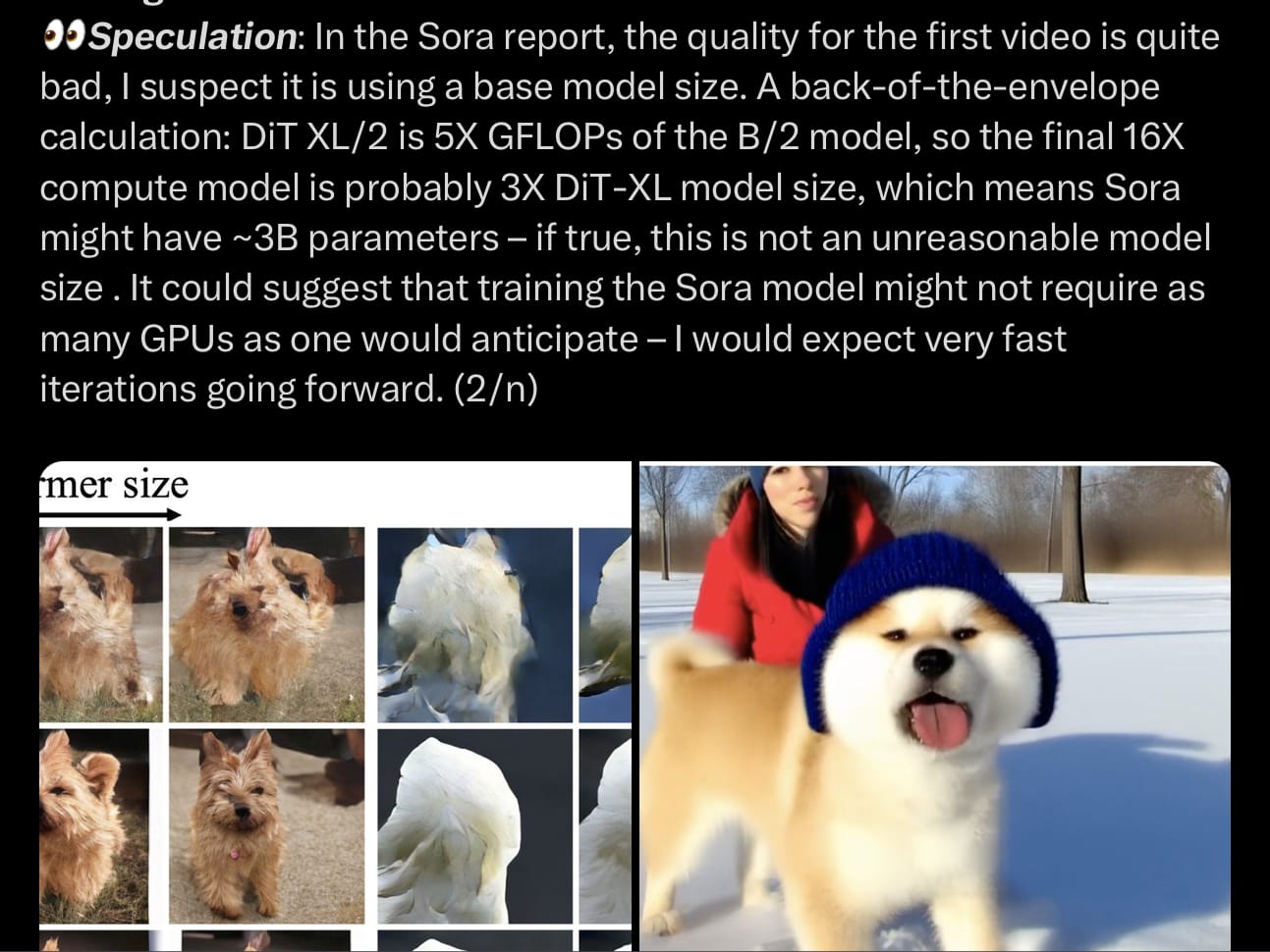
People in the comments speculating that it could be 3B or 6B parameter model, in which case….we could probably train one ourselves given the right data. Let me know if you want to take a stab - Oxen.ai is collecting and gathering a large video dataset we will open source soon.

Feel free to email hello@oxen.ai if you are interested in collaborating.

Next Up

To continue the conversation, we would love you to join our Discord! There are a ton of smart engineers, researchers, and practitioners that love diving into the latest in AI.

Join the oxen Discord Server!

Check out the oxen community on Discord - hang out with 616 other members and enjoy free voice and text chat.

Discord

If you enjoyed this dive, please join us next week live! We always save time for questions at the end, and always enjoy the live discussion where we can clarify and dive deeper as needed.

All the past dives can be found on the blog.

The live sessions are posted on YouTube if you want to watch at your own leisure.

Best & Moo,

~ The herd at Oxen.ai

Who is Oxen.ai?

Oxen.ai is an open source project aimed at solving some of the challenges with iterating on and curating machine learning datasets. At its core Oxen is a lightning fast data version control tool optimized for large unstructured datasets. We are currently working on collaboration workflows to enable the high quality, curated public and private data repositories to advance the field of AI, while keeping all the data accessible and auditable.

If you would like to learn more, star us on GitHub or head to Oxen.ai and create an account.

Arxiv Dives

ArXiv Dives - Diffusion Transformers