How We Cut Inference Costs from $46K to $6.5K Fine-Tuning Qwen-Image-Edit
At Oxen.ai, we think a lot about what it takes to run high-quality inference at scale. It’s one thing to produce a handful of impressive results with a cutting-edge image editing model,but an entirely different challenge when you’re generating millions of images. At that scale, efficiency and cost become critical. Shaving even a few seconds off each inference can translate into tens of thousands of dollars in savings.
So, in true Oxen fashion, we rolled up our sleeves, ran the numbers, and experimented with optimizations to see just how far we could push both performance and efficiency of image editing models.
This is the story of how we brought a $46,800 image-generation project down to just $7,530, while still keeping the quality needed for a real commercial catalog. If you'd prefer to watch the video version, we do a live stream on Friday's with the community where we talk through the gnitty gritty details:
Also, don’t hesitate to join our Discord. Our community is always excited to dive into AI/ML, share ideas, and swap lessons learned from real-world projects.
The Task: Generating a Product Catalogue
Recently, we had an AI-native consulting firm named AlliumAI come to us because needed to generate a catalog of furniture. The product catalogue had a variety of items such as desks and cabinets and different color swatches that needed to be used for these items.
The problem is, there are 192 different color combinations, and ~6000 different pieces of furniture. This means there are ~1.2 million different combinations that users can view and select from, way too many for a photoshoot, thats where we come in.
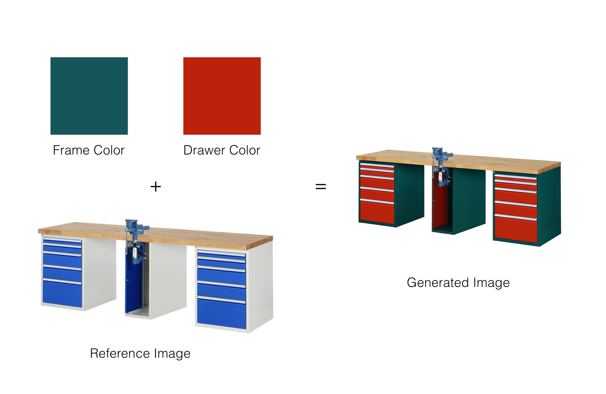
For context, here are some example of the color swatches:

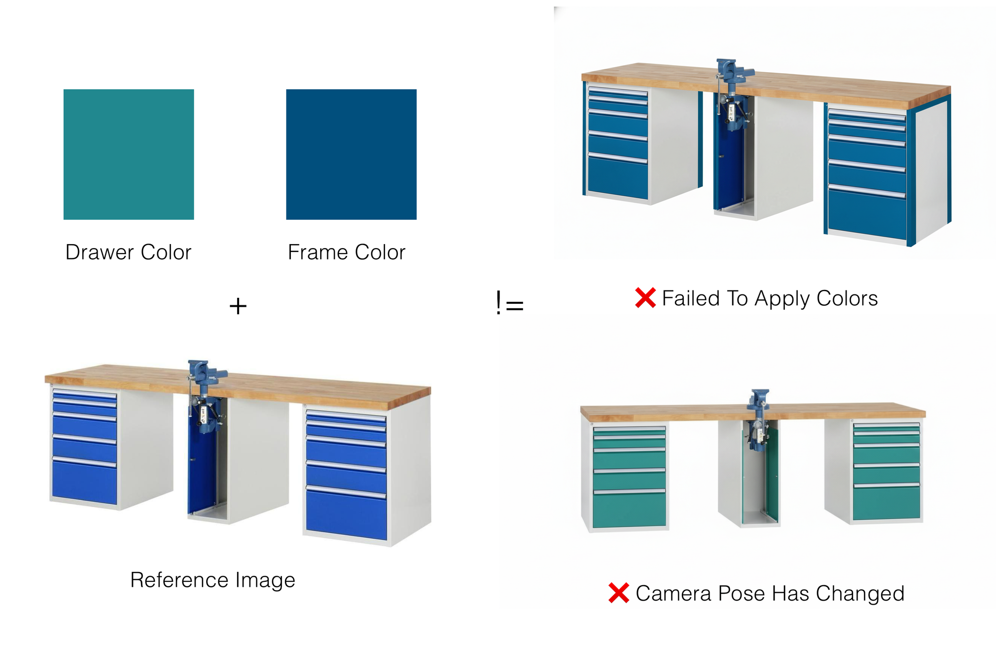
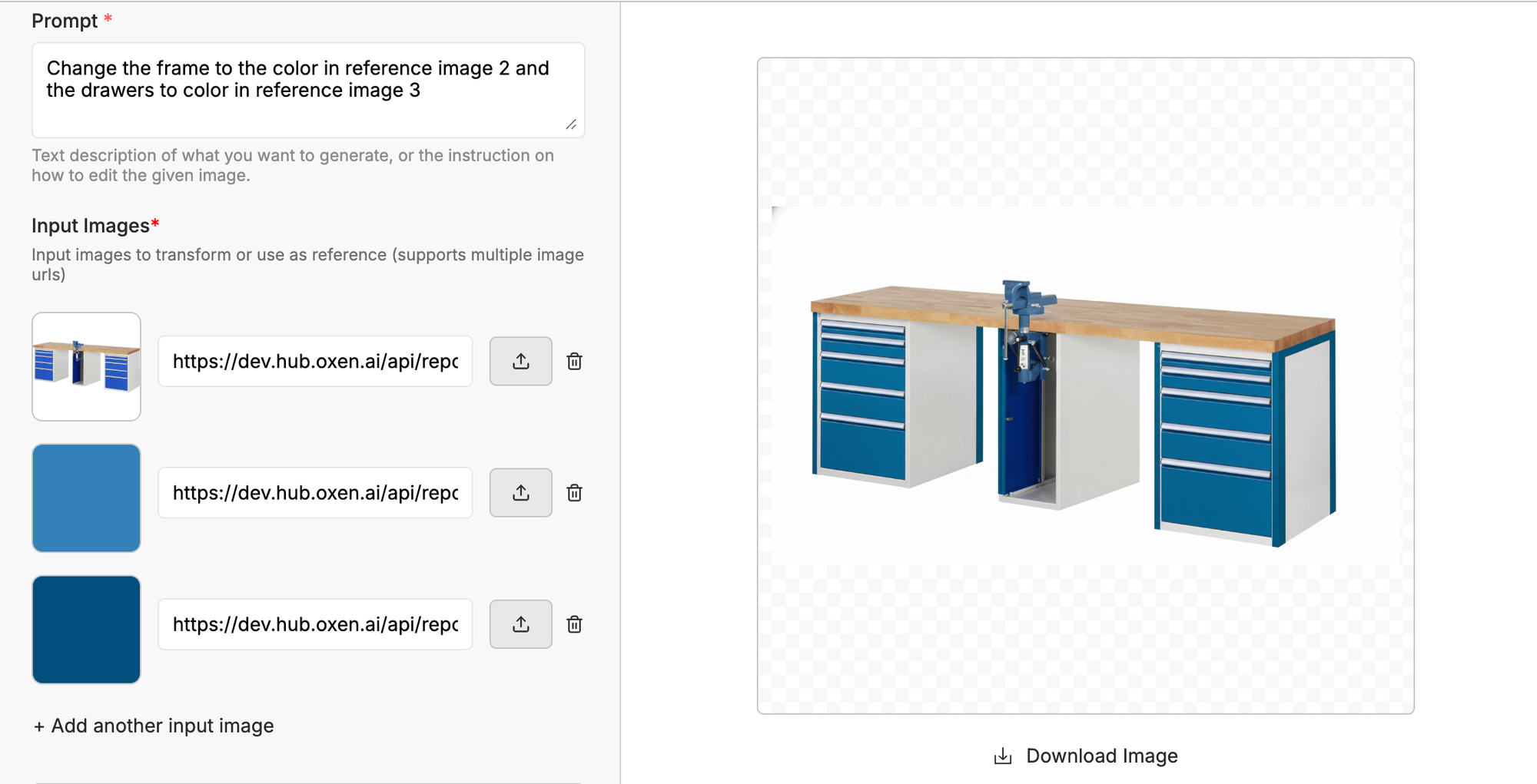
At first glance, this seems like the perfect task for SOTA image editing models like OpenAI's gpt-image-1 and Google's Nano-Banana, that take in multiple reference images and a prompt and generate a new image. Some quick tests in the Oxen.ai playground were pretty promising...
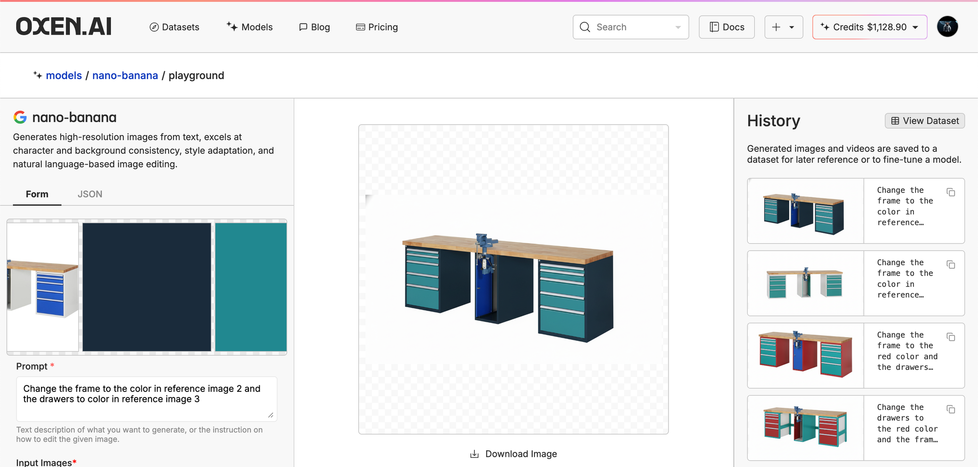
But they are far from perfect. If you look in the history panel on the right, there are a lot of result images that are not production ready, rotated desks and incorrect colors are unacceptable for this particular use case.
When we did the back-of-the-napkin math, it became clear that this approach was far too expensive for our budget. At $0.039 per image with Nano-Banana, generating all 1.2 million images would cost around $46,800. Clearly, we had some work to do.
We were optimizing for two key variables: price and consistency. Fortunately, fine-tuning offered a promising path forward, it’s often an excellent way to balance quality with efficiency in large-scale generation tasks.
Step one: Data Collection
While Nano-Banana and GPT-Image-1 aren’t perfect for this task, they’re a powerful way to generate manually curated, labeled data.
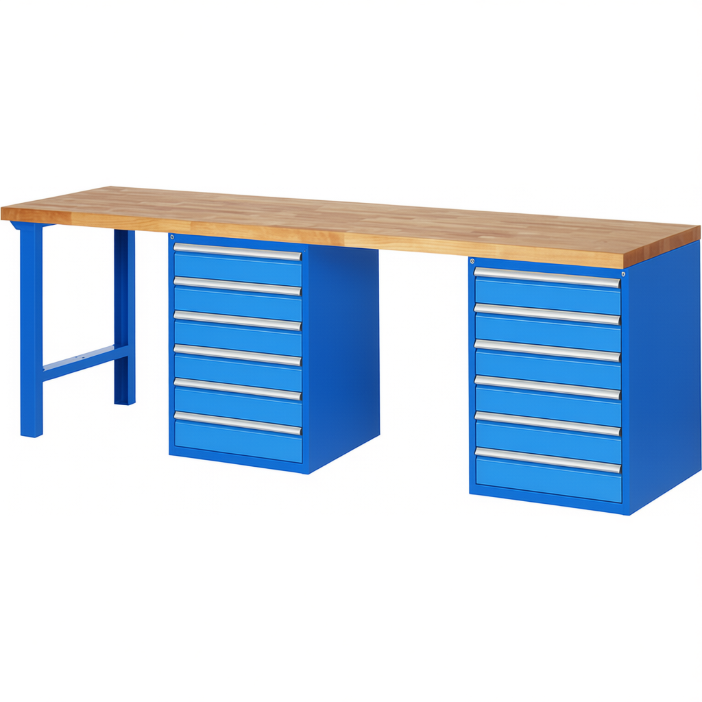
After the first round of synthetic data generation, our client realized the results weren’t yet production-ready. They brought in editors to manually refine the images in Photoshop, transforming the imperfect generations into high-quality training data. Some color combinations proved particularly challenging for the base models, for example, the light blue and dark blue desk shown below.
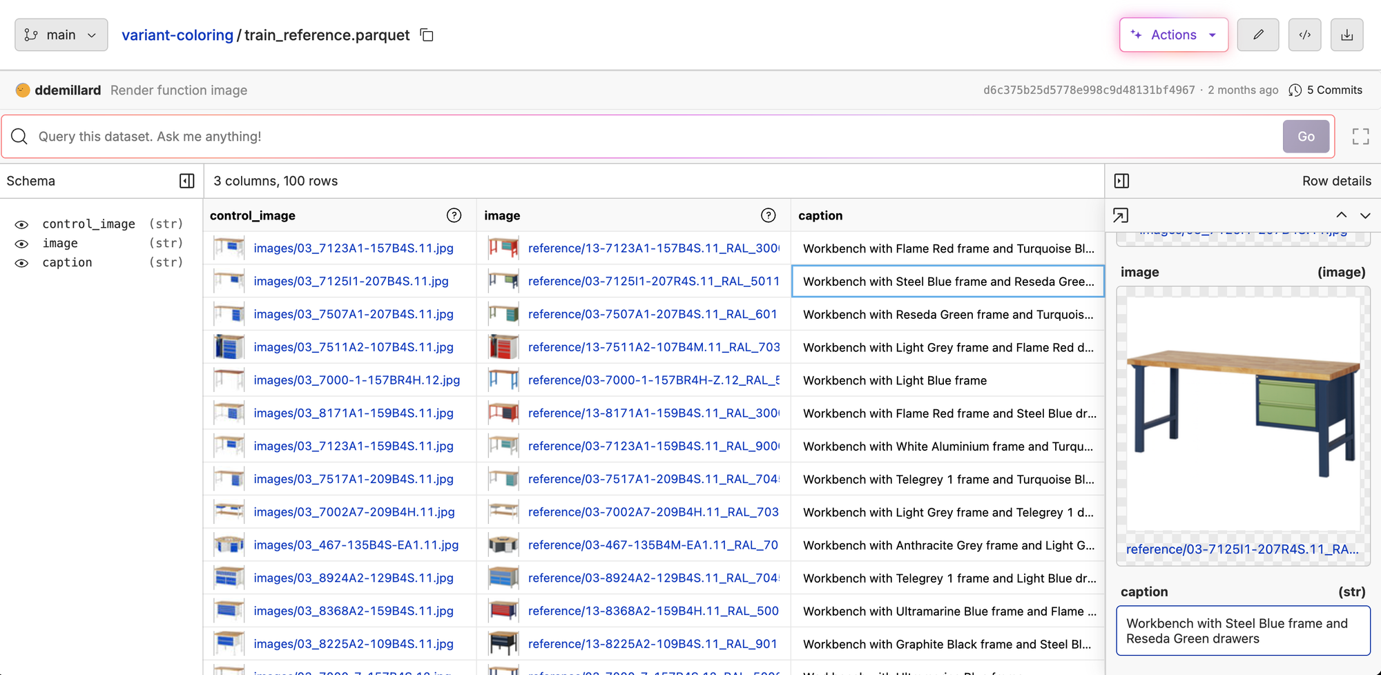
By the end of the process, we had a nice dataset consisting of every color combination on a subset of the pieces.
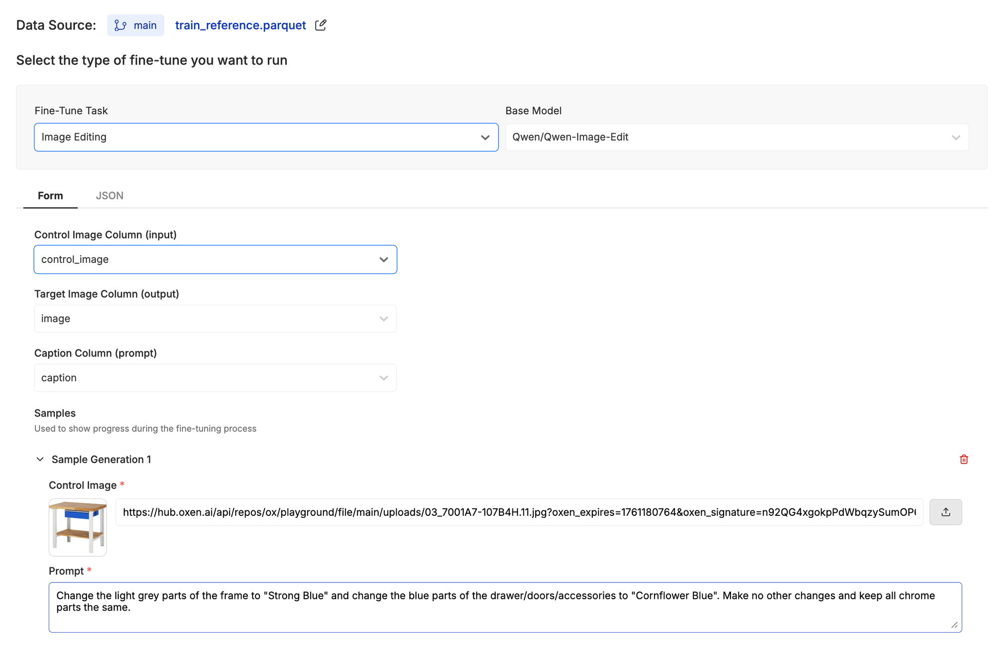
Step Two: Fine-Tuning
Our goal at Oxen.ai is to let anyone fine-tune any state of the art model, with as few clicks as possible. We handle the storage and compute infrastructure, so you can focus on what matters, the end product.
Using the base Qwen-Image-Edit, we got some pretty promising results. This showed us that a fine-tune could be effective, so we decided to run a small experiment: how far could we get with just 100 examples? The dataset was intentionally small, just enough to illustrate our workflow.
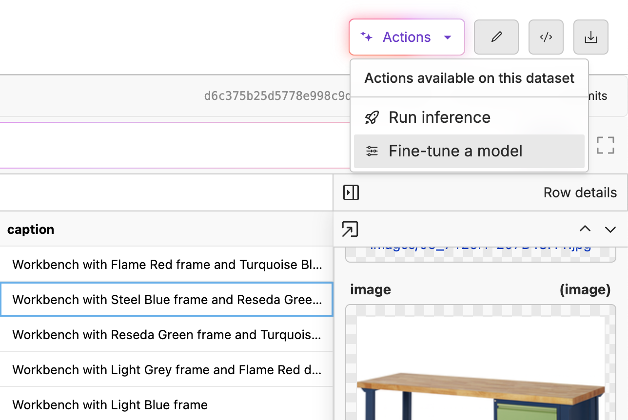
Once we got this dataset into Oxen, we started a fine-tune with a single click.
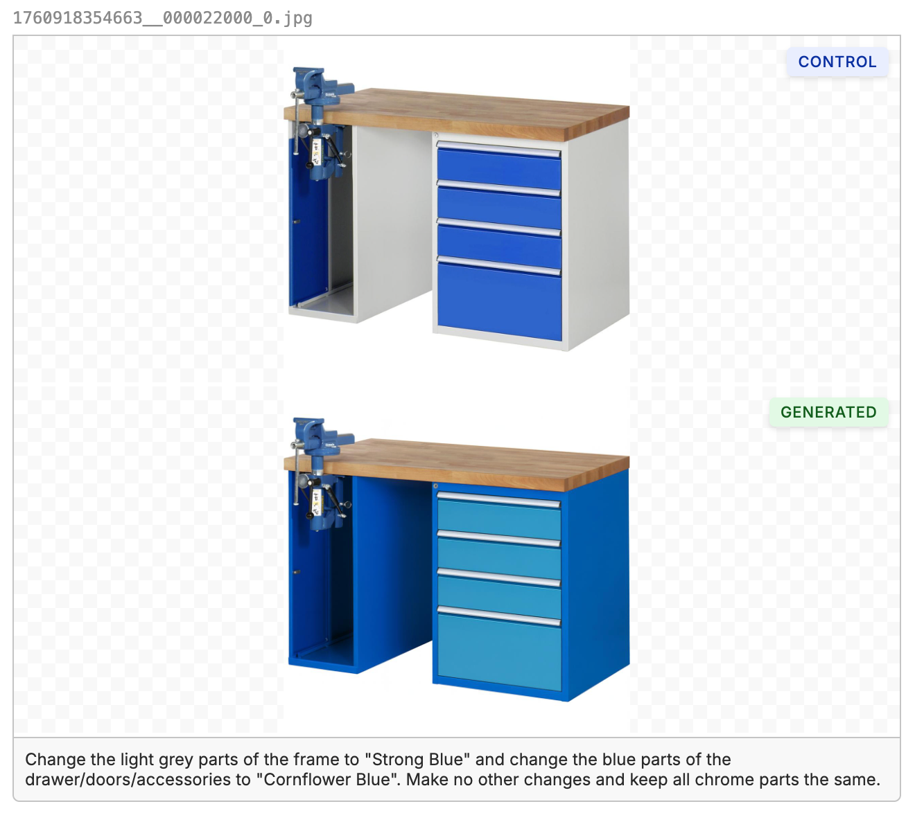
This first fine-tune cost us about $8 and took roughly 2 hours to complete. Looking at some of the test samples that were generated during training, the model was already generating very good results with some of the color combinations the base models struggled with!
We then scaled up the dataset to over 1,000 examples. Quality-wise, we were satisfied with the generation our fine tuned model was outputting. But there was still one big problem: cost at scale.
Step Three: Cost Optimization
Here at Oxen.ai we love open source models, so we used Qwen-Image-Edit and its Apache 2.0 licenses to do some fancy optimizations to reduce inference time. And as we all know, fast inference is cheap inference.
Qwen-Image-Edit is a decently large model, taking up about 60 GB of VRAM. This means that to run the unquantized model we need an H100 gpu, also, from our initial experiments, each image took about 15 seconds to generate. Knowing an H100 on Oxen.ai costs $4.88/hour, we can do some back-of-the-napkin math:
Time per image: 15 s → 18,000,000 seconds total
Total hours: 18,000,000 ÷ 3600 ≈ 5,000 hours
Total Cost: 5,000 × $4.88 ≈ $24,400
This is a great start, we dramatically improved performance and decreased costs compared to the previous estimate of $46,800, almost a 48% reduction!
The bad news is that $24K still was outside the budget for this project. We were closer, but not quite there. That meant we needed to get creative with these optimizations. We identified three main levers we could pull:
1) Pre-compilation of the PyTorch graph
2) Using a Lightning LoRA
3) Quantizing the model
We'll walk through each one, and the costs and benefits of each.
Option 1: Compile the PyTorch Graph
Our first idea was to use torch.compile, which can optimize model execution by fusing operations together and reducing Python overhead.
The benefit? Potential speedups with almost no code changes.
The risk? Compiling a model as large as Qwen-Image-Edit can take a while the first time, so it does increase cold boot time.
But in this case, the tradeoff made sense, we were going to use a single model to generate 1.2 million images, so paying a one-time compile cost upfront was absolutely worth it if it shaved even a few seconds off each image generation
All we had to do to test this was add these 2 function calls.
pipe.transformer = torch.compile(
    pipe.transformer, mode="max-autotune-no-cudagraphs", dynamic=True
)
pipe.vae.decode = torch.compile(
    pipe.vae.decode, mode="max-autotune-no-cudagraphs", dynamic=True
)
transformer is the text-to-latent module, i.e., it takes the text prompt and produces the latent representation. This usually contains a huge number of transformer layers, so it’s compute-heavy and benefits a lot from compilation.
Vae.decode is the decoder of the VAE that converts the latent representation into an actual image. It’s also heavy and benefits from compilation.
The compilation itself took about five minutes (roughly 300 seconds). That might sound like a lot, but the payoff was worth it: we were able to drop the per-image generation time from 15 seconds down to 12.46 seconds.
So here’s what the math looks like:
Time per image: 12.46 s → 14,952,000 seconds total
Total hours: 14,952,300 ÷ 3600 ≈ 4,154 hours
Total Cost: 4,154 × $4.88 ≈ $20,271
In other words, we were able to generate very high-quality images and cut costs by another ~$4K compared to the uncompiled baseline. There’s still a bit of optimization left on the table, but this gets us a lot closer to where we want to be.
Option 2: Using a lighting LoRA
When we started looking for ways to further optimize our throughput, we came across this LoRA module:
This LoRA lets us generate images using fewer inference steps without compromising too much on quality. Fast inference means cheap inference, but we have to be careful, fewer steps can sometimes hurt the fidelity of the output. The key is finding the right balance between speed and quality.
(Quick side note: in a diffusion model, “steps” refer to the number of denoising iterations the model goes through to turn random noise into a coherent image. More steps usually give higher-quality images but take longer, while fewer steps are faster but can risk rough or unfinished outputs. Using a 4-step LoRA means the model only needs 4 denoising iterations instead of the usual 20 or more)
Since we were already using a LoRA trained on our toy car dataset, we needed to stack both our custom LoRA and this Lightning LoRA for the experiment. Here’s how we set it up:
pipe.load_lora_weights(
    "Qwen-Image-Edit-Lightning-4steps-V1.0-bf16.safetensors",
    adapter_name="lightning_lora",
)
pipe.load_lora_weights("model.safetensors", adapter_name="desks", prefix=None)
pipe.set_adapters(["desks", "lightning_lora"], adapter_weights=[1.0, 1.0])
Because we chose the 4-step Lightning LoRA, we also needed to adjust the number of inference steps in the generation call:
image = pipe(
    image=input_image,
    prompt=prompt,
    num_inference_steps=4,
    true_cfg_scale=4.0,
    generator=torch.Generator(device="cuda").manual_seed(42),
).images[0]
The best part, this only took 4.63 seconds per image.
Continuing with our back-of-the-napkin math, this means:
Time per image: 4.63 s → 5,556,000 seconds total
Total hours: 5,556,000 ÷ 3600 ≈ 1,543 hours
Total Cost: 1,543 × $4.88 ≈ $7,530
Compared to our previous setup at 12.46 s per image, this is a massive reduction in both time and cost, and the image quality is still very respectable.
Just to keep track, we were able to bring our total inference cost down from $46,800 to $7,530 while maintaining very good image quality. Not bad at all! This is already a pretty excellent improvement, but we still had one more trick up our sleeve…
Option 3: Quantization
Even after stacking LoRAs and cutting inference steps, we still had one more lever to pull: quantization.
The goal here was to make our model take up less than 40gb of vram so we could run it in a smaller/cheaper GPU like the H100MIG
Quantization is a technique that reduces the precision of the numbers the model uses, from full 32-bit floats down to 16-bit, 8-bit, or even lower. The idea is simple: smaller numbers mean less memory usage, faster computation, and less GPU time, ideally without drastically affecting the output quality.
In our pipeline, we experimented with lower-bit representations for both the transformer and the VAE. In theory, this should allow faster image generation and less memory needs.
To do this, we just added this code:
quantization_config = DiffusersBitsAndBytesConfig(
    load_in_8bit=True,
    llm_int8_threshold=6.0
)
transformer = QwenImageTransformer2DModel.from_pretrained(
    model_id,
    subfolder="transformer",
    quantization_config=quantization_config,
    torch_dtype=torch_dtype,
    device_map="cuda",
)
quantization_config = TransformersBitsAndBytesConfig(
    load_in_8bit=True,
    llm_int8_threshold=6.0,
)
text_encoder = Qwen2_5_VLForConditionalGeneration.from_pretrained(
    model_id,
    subfolder="text_encoder",
    quantization_config=quantization_config,
    torch_dtype=torch_dtype,
    device_map="cuda",
)
print_memory_usage("After loading text encoder")
pipe = QwenImageEditPipeline.from_pretrained(
    model_id,
    transformer=transformer,
    text_encoder=text_encoder,
    torch_dtype=torch_dtype,
    device_map="cuda"
)
Now, lets talk about the results:
Not bad at all.
The good news? VRAM usage dropped to 33 GB, well below our 40 GB target and far from the 60 GB the unquantized model requires.
The bad news? Inference slowed down to 14.85 seconds per image. In this case, the memory savings were completely offset by slower generation. To achieve the same cost as our optimized pipeline, we’d need to run this quantized model on a GPU that’s three times cheaper than our base H100 and still has at least 40 GB of VRAM, and unfortunately, no such GPU exists.
Why was it slower even after quantization?
Quantization reduces memory usage by using lower-precision numbers (like 8-bit instead of 32-bit), but it doesn’t automatically make inference faster. Here’s why in our case:
Hopper GPUs (H100) are optimized for low-precision computation, but only if the framework and kernels actually leverage them efficiently. Some layers, or LoRA adapters, may still run in higher precision or fall back to FP16/FP32, which adds overhead.
Quantizing activations and weights involves scaling, de-scaling, and rounding operations, which can slow things down, especially for small batch sizes or few inference steps.
Instead of using BitsAndBytes to quantize the model at runtime, we used a pre-quantized version of the Qwen-Image-Edit transformer layer: Qwen-Image-Edit-int8wo.
This version has its layer weights pre-converted to int8, eliminating the runtime overhead of converting between precisions during inference. While the exact method isn’t publicly documented, this pre-quantization was likely done using a weight-only int8 quantization workflow, such as AWQ or GPTQ, which are commonly used to generate fast, high-performance weights for transformer-based models.
To do this we just have to add the following code:
from diffusers import AutoModel

quantization_config = DiffusersBitsAndBytesConfig(
    load_in_8bit=True,
    llm_int8_threshold=6.0
)

transformer = AutoModel.from_pretrained(
    "dimitribarbot/Qwen-Image-Edit-int8wo",
    torch_dtype=torch_dtype,
    use_safetensors=False
)

pipe = QwenImageEditPipeline.from_pretrained(
    "Qwen/Qwen-Image-Edit",
    transformer=transformer,
    torch_dtype=torch_dtype
)

pipe = pipe.to("cuda")
Small caveat: we only quantized the transformer layer, which is the largest layer in the model. Since we didn’t quantize the other layers, notably the VAE, we lose a bit of memory optimization.
The good news? This model requires 39 GB of VRAM, meaning it can safely run on an H100 MIG. Even on this smaller GPU, using this pre-quantized transformer layer, each image generation takes around 10 seconds!
Let’s pull out our napkin again, knowing an H100 MIG costs $1.95/hour on Oxen:
Time per image: 10 s → 12,000,000 seconds total
Total hours: 12,000,000 ÷ 3600 ≈ 3,333 hours
Total Cost: 3,333 × $1.95 ≈ $6,500
Yes! That’s a 13.7% reduction from our previous $7,530 estimate, and a whopping 85.9% improvement from our original $46,000 estimate, all while maintaining production-level quality. Long live fine-tuning! 🚀
Inference Time
We haven’t talked about a very important aspect of this workflow: how long it actually takes to generate all of the images. We’re generating 1,200,000 images, and even if we managed to lower the per-image generation time from roughly 15 seconds down to about 4 seconds, running the entire workflow on a single GPU would take:
4 s × 1,200,000 images = 4,800,000 seconds
4,800,000 ÷ 3600 ≈ 1,333 hours
That’s over 55 days on a single GPU, obviously unreasonable.
Fortunately, with Oxen.ai’s async inference serving, we can run multiple GPUs in parallel. Using 16 H100 GPUs, the total runtime drops to:
1,333 hours ÷ 16 ≈ 83 hours
That’s just under 3.5 days, making the generation of 1.2 million images feasible in practice. And the best part? Oxen.ai handles all of the GPU management for you, so you can just trigger the run and not have to worry about infrastructure management.
If you're curious about running a workload this large, feel free to reach out at hello@oxen.ai, we'd be happy to help.
Conclusion
The biggest takeaway from this project is that meaningful performance and cost optimizations are possible when you combine multiple strategies thoughtfully. By leveraging open-source models, fine-tuned LoRAs, and techniques like compilation, low-step inference, and quantization, we improved image quality while cutting GPU time by over 6× and reducing cost from 46,800 to just 6,500.
Just as importantly, this workflow shows that scaling to massive datasets doesn’t have to be prohibitively expensive. With asynchronous GPU serving and the right optimizations, teams can run huge amounts of inference efficiently while freeing resources for other parts of the project.
The key lesson is that optimization is multi-dimensional: it’s not just about making one component faster or cheaper, it’s about stacking model-level, algorithm-level, and infrastructure-level improvements to maximize overall performance and efficiency.
That’s our bread and butter here at Oxen.ai. We love finding and sharing these techniques through our fine-tuning, deployment, and inference tools, so you can focus on solving your or your clients’ real challenges while we handle the heavy lifting.
Don't hesitate to reach out if you have any questions! Also, if you're working on a project where you could use our expertise or are interested on using Oxen to run fine tunes or inference at scale feel free to create an account on Oxen.ai, send us an email at eloy@oxen.ai or join our discord here!
Don’t be shy, reach out if you have any questions! If you’re working on a project where our expertise could help, or want to use Oxen to run fine-tunes or inference at scale, go ahead and create an account on Oxen.ai, shoot us an email at eloy@oxen.ai, or hop into our Discord community (we love answering questions and chatting with folks!)
Until next time, Bloxy out!